How To Freeze Rows And Column In Excel 2016 1

How To Freeze Rows And Column In Excel 2016

Working with a big spreadsheet you will want to be able to see the header, usually top row and first column although you scroll the bar on the side or bottom section. This is what called freeze rows and columns.
In Excel 2016 we can freeze first row, first column, row and column and we can unfreeze all of them to make the spreadsheet back to the original position.

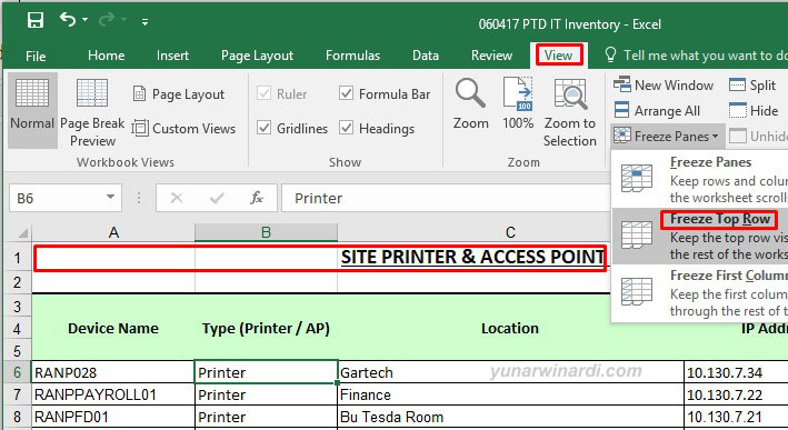
Freeze First Row or Top Row

Click View-Free Top Row and your row number 1 will stay visible when you slide to the bottom. To freeze the first third rows, click on any column in the fourth row, click View-Freeze-Freeze Panes.

freeze first row

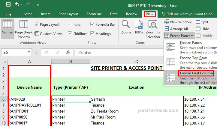
Freeze First Column

Click View-Freeze First Column make column A stay visible when you slide left and right. To freeze the first third column click the whole fourth column by clicking column’s header, for example, column header E. Click-View-Freeze Panes.
freeze first column

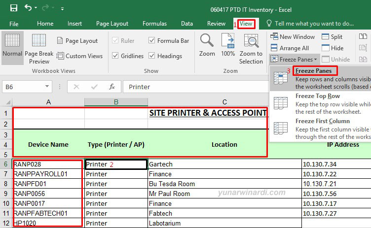
Freeze Certain Rows and Column

Click on the cell just under the row and next to columns you want to freeze. Click View-Freeze panes will make the rows and columns above and besides current active cursor keep visible or not scrollable.
freeze rows and column

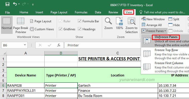
Unfreeze Panes

Unfreeze panes will make all rows and columns in current sheet scrollable, or back to original position.
unfreeze row and column

In the sample above I am using Excel 2016 but excel in another version will be the same except the location of Freeze panes slightly different.

How useful was this post?

Click on a star to rate it!

Average rating 0 / 5. Vote count: 0

No votes so far! Be the first to rate this post.

Similar Posts

Leave a Reply

Your email address will not be published. Required fields are marked *